Over the decades, we’ve learned how to exploit radio waves across the entire frequency spectrum; it’s hard to believe that, in years past, many of these frequencies were considered useless. Each frequency band dictates antennas of a different length and often with unusual requirements. To help find the best solution for any application, engineers turn to electromagnetic simulations. They use modelling software not only to refine the performance of existing antennas, but they’re also trying to find ways to meet novel requirements with new materials – and are also studying the use of antennas for new applications. This article will give you a flavour for some of these fascinating designs.
From small to large
First, however, note that a number of modelling techniques can solve Maxwell’s Equations, which are the base of any electromagnetic study: finite elements (FE), method of moment (MoM), finite-difference time-domain (FDTD) and many others – and software suppliers will argue the pros/cons of one over the other. With its HFSS software (High-Frequency Structure Simulator) for electromagnetic field simulation, for instance, the Ansoft division of Ansys has opted for the finite element method because, according to HFSS product manager Matt Commens, it’s very ‘general purpose’ without any particular areas where it’s weak: ‘We can analyse an antenna integrated into a small package, such as a mobile phone, or work on something as large as antenna placement on an aircraft,’ he says. ‘The scale of what we can study is of many orders of magnitude.’ He also points to the package’s use of tetrahedrons in the mesh, which can precisely fill any arbitrary geometry, its adaptive meshing and optimisation capabilities, all without any hand-tweaking. For him, such software has moved from being an analysis tool to a design tool where the engineer defines the problem parameters and lets the software apply its magic.
Commens also explains that people now want antennas in a physical package, which would have been considered impossible just 10 or 15 years ago. A great example comes from RFID technology – the use of radio tags on everything from articles of clothing to pallets in a warehouse. An interesting development is the RFID printer. This unit receives barcode information, which it prints on labels that have embedded chips/antennas and also encodes the data into the chips. Here, an interesting problem is that the radio links must work well enough – but not too well; when information is imprinted into a target RFID chip, a radio link’s behaviour should be strong enough to be detected at the target chip, but not strong enough to imprint information on other chips close by on the same label roll. Designing antennas for such unusual constraints becomes far easier with simulation software.
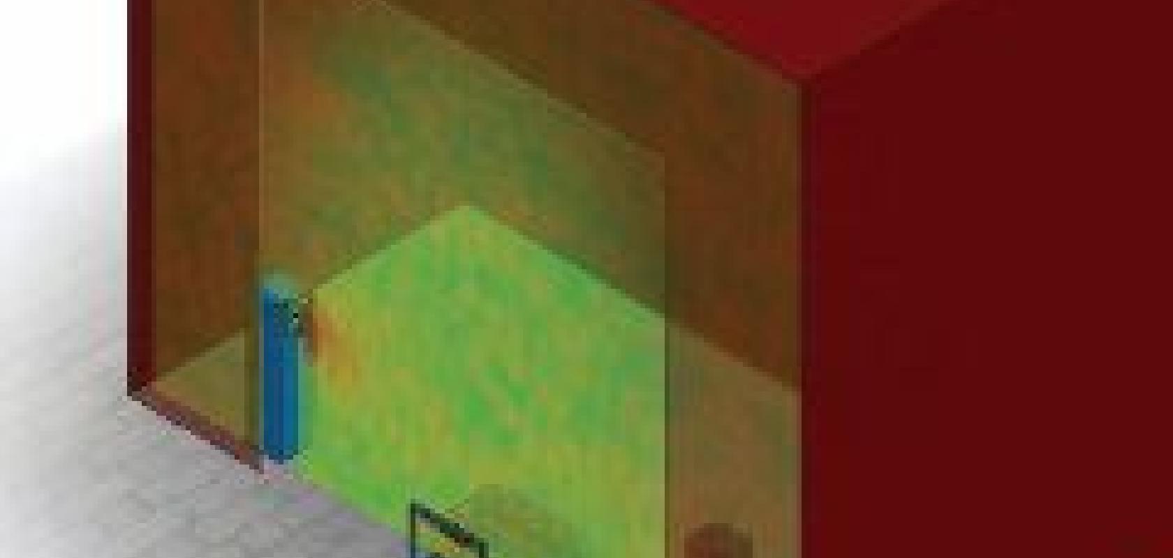
The image (top) shows a pallet entering a warehouse with multiple packages, each with multiple RFID tags. The reader antennas on the pedestals to either side of the doorway first excite the RFID tags and then read the information from them to track the movement of goods. The red, yellow, green mottled image represents the electric fields at the cut plane connecting the two reader antennas. An engineer can use such information to understand how the fields are scattered in their particular environment. This is overall a relatively large simulation that was enabled and made considerably more efficient with recent HPC enhancements to HFSS.
At the other extreme, adds Commens, is large-scale analysis; people generally want to put their antenna on something, whether it be a military vehicle or even a spacecraft. In these situations, simulations tend to be very large, so in HFSS 12.0 Ansoft released its domain decomposition matrix solver. This HPC technology means users are no longer restricted to fitting a simulation into the memory on one machine, and he reports that the scale of simulations thus increases by a factor of 10 to 100. With these larger designs, though, come new concerns when modelling the environment around the antenna. Thus, HFSS 12.1, just announced, adds 3D MoM techniques – which, Commens explains, are very good in dealing with a large, open radiating structure with many conductive elements around it (in comparison, FE shines in applications such as a radomes with its many dielectrics).
GPS antennas with precise phase
Such a situation with conductive elements presented a potential problem with the GPS antennas for satellites being designed for the European Space Agency’s Swarm mission, scheduled for deployment this year. The Swarm project will provide the best-ever survey of the Earth’s geomagnetic field and its evolution over time. It consists of three satellites in three different polar orbits between 400 and 550km in altitude.
The two GPS antennas on each Swarm satellite must be able to take readings from GPS satellites and determine POD (precise orbital determination) to within a few centimetres compared to five to 10 metres on earth; this level of positioning accuracy is crucial for the Swarm satellites to acquire useful data with its specialised instrumentation. These antennas must be positioned very carefully; to achieve the required accuracy, there must be very little phase distortion, which could arise from reflections off solar panels and other parts of the satellite. This signal scattering and the resulting reflections can disturb GPS performance and introduce errors, but in this application the engineers must know the exact radiation pattern. Further, there was limited room for the antennas on the satellite.

CAD model of the Swarm satellite (left), where the two GPS antennas are located on the upper part of the rectangular panel; the efield simulation (right) shows the surface currents on the satellite centred around the antennas.
To evaluate the spacecraft’s impact on the antennas and help in their placement, engineers at RUAG Space AB in Sweden performed the analysis and design work. Following the simulations came measurements on a mock-up for verifying antenna performance. For their analysis, they turned to efield software from the Swedish company of the same name. In this case, the software runs the MLFMM (Multilevel Fast Multipole Method) solver rather than the MoM (Method of Moments) solver. MLFMM is used to speed up matrix-vector multiplications that are the dominating operation in the iterative solver used to solve the MoM matrix system. MLFMM is based on a 3D partition of the object into boxes of different size at different levels so that a fast matrix-vector multiplication can be computed. For a typical satellite application with 100,000 unknowns, the MoM method requires 150Gb of memory whereas the MLFMM approach requires far less, at approximately 2Gb.
The implications are significant because, explains RUAG engineer Per Ingvarson, while it was always possible to simulate isolated components, the team can now simulate small components as well as the entire spacecraft structure and better see how the GPS antennas interact with the satellite itself.
Antennas for all conditions
As technology has advanced, says Dr Christopher Penney, co-founder of Remcom Inc, tools have been developed that go beyond merely analysing existing antennas to tools that help design them from scratch. Users select basic structures with variable dimensions, size, constraints and performance goals, then the software iterates until it finds the best possible design. Much of the burden of setting up and repeatedly running simulations is removed, since the calculations are performed in part without user intervention. When combined with solvers that run extremely fast on GPUs, turnaround time can be significantly reduced.
Consider an example using Remcom’s XFdtd Release 7. A recent project had the task of designing a small wideband, vertically polarised antenna for use in near-to-ground situations that would radiate a uniform pattern in the horizontal plane. The antenna application was to transmit data from a ground sensor that monitors movement, such as road traffic, to a remote monitoring station. It is intended for mounting atop a small cylindrical sensor, approximately 23cm tall with a radius between 10 and 15cm. The system’s wide bandwidth – from 225 to 500MHz – ensures propagation in difficult conditions where environment, interference and jamming attempts might render some frequencies unavailable.
Several models were investigated, and the best candidate proved to be a broadband sleeve monopole. A prototype was fabricated based on early simulations that provided acceptable performance in free space. However, when the antenna was placed on the ground as it would in actual use, performance did not meet the design goals for all frequencies.
Using the PSO (particle swarm optimisation) technique, Remcom started a redesign to optimise it for four situations: the antenna in free space, on dry ground, on medium ground and on wet ground with the goal of finding one antenna that meets performance specifications for all these cases.
In other test cases for much larger geometries that use significantly more memory that this design, running the PSO simulations using an Nvidia Tesla GPGPU card is more than 100x faster than a single processor.
And, while the computational performance gain for this antenna design is less than half that amount, it is still significantly faster than an eight-core processor. This increase is considerable given that during the optimisation process, several hundred simulations were run for each trial, and about 40 different trials were made.
After reviewing results from the four cases, it became clear that the designs optimised just for free space and dry ground are quite different than those for wet and for medium ground.
Attempting to average the parameters from all these cases results in a design that doesn’t perform well everywhere. However, because the free-space and dry-ground cases were somewhat flexible in their design, the engineers found that the average of the wet- and medium-ground cases performs suitably well for all situations.

Original BBSM antenna (right) and a design optimised for use on various ground conditions (left) as calculated with XFdtd Release 7 from Remcom.
The nearby figure shows a comparison of the original and final antenna designs; the optimised unit is shorter than the original with a higher sleeve and much larger top-hat radius. Their shapes might seem similar, but performance is vastly different. The return loss and VSWR for this final design are within the design limits for nearly all frequencies.
Antennas for digital transmissions
Scientific software is also helping broadcast network operator Arqiva model antennas and analyse systems. That firm handles all land-based transmissions for UK television stations, including the new digital networks, as well as wireless provision for cellular, wireless broadband, voice and data services.
‘In order to fully understand how a network functions and the nature of the maths behind it, we need something to quickly and simply check what’s happening,’ says Arqiva senior technologist Karina Beeke. For that, they turn to Maple software with its features such as space curve, aptitude, curve fitting and the ability to rotate and zoom into elements.

A plot created with Maple’s SpaceCurve function to visualise OFDM carriers. Each line radiating from the main horizontal axis represents one carrier with the bolder/thicker carriers being the pilot carriers.
More specifically, Beeke uses Maple to analyse the OFDM (orthogonal frequency division multiplex) signals for digital TV and radio where reflections off objects, such as buildings, create multipath effects. The software’s plotting routines visualise what is happening and improve the engineers’ understanding.
It also aids in antenna matching, which is useful in creating a model in another simulation package for investigating the heating of a body in an RF field. Various parameters from the antenna feedpoint were used as inputs to Maple to optimise the match, which is necessary to ensure that the simulation maximised the power radiated by the antenna; otherwise they might underestimate the heating effect.
Sending radio signals into the ground
Rather than the design of an antenna, this final application examines an unusual application of very-low-frequency radio waves: seabed logging. Researchers have developed methods using simulation software to help identify hydrocarbon reservoirs prior to drilling.
Dr Andreas Aspmo Pfaffhuber, discipline leader in geophysics at the Norwegian Geotechnical Institute (NGI), explains that well-known seismic survey methods using acoustics can indicate what an undersea geologic formation looks like, but they can’t guess at what it might contain.
Meanwhile, a new technique has come into use whereby an exploration vessel drags a long wire antenna called a horizontal electric dipole (HED), perhaps 200m long, 30m or 40m above the ocean floor. It transmits signals in the range 0.1 to 10Hz with extremely high power up to more than 1,000A. The interactions of the electromagnetic fields with the structures underneath the sea bed are evident in the spatial development of the EM fields, which are sampled by a series of perhaps 20 receivers situated in a line along the sea bottom.
A critical aspect is that the resistivity of sediments above and below a hydrocarbon reservoir is in the range of a few ohm-meters, whereas the resistivity of hydrocarbons can be 10 to 100 times higher. Thus, by measuring the amplitude and phase of the received signal, geophysicists can identify locations with a high probability of containing reserves. Each survey run results in a 2D section, so multiple runs are necessary to develop a full 3D representation.
To dig this information from the raw data requires sophisticated filtering and post-processing. For instance, changes in sub-sea geology or strong sea floor topography can lead to effects very similar to those from a reservoir. One analysis tool used by NGI researcher Tore Ingvald Bjørnarå is Comsol Multiphysics, with which he performs both forward and inverse modelling. In forward modelling, the goal is to determine whether it would be worthwhile doing a detailed survey of a given area. He starts with seismic and bore-hole data to get a good idea of the electromagnetic properties of the layers in the subsurface.

Comsol Multiphysics results of a seabed modelling study, which represents just one slice in the 2.5D geometry. It is taken along one receiver line and shows the spatial distribution of the transmitted EM field strength as it interacts with a hydrocarbon reservoir (rectangles in the centre of the line).
He then makes certain assumptions about the sea water and the hidden hydrocarbons and runs a simulation in a Comsol Multiphysics model that he has developed. The resulting data curves are examined to see if it is likely that a survey would be able to detect any hydrocarbons.
In an inverse study, you start with the response curves from an electromagnetic study where you don’t know the properties of the fluids involved. Here he runs a Comsol model to find the best fit for the curves assuming various material properties. Tight integration with existing geological information is crucial to find a realistic solution of the ill-posed inversion problem.
These inverse models are very complicated, he adds, because there are so many unknown parameters, and the Comsol models can thus be very large. On a 64-bit PC he is limited by memory and so he is excited to see what benefits the new cluster version of Comsol will bring. For one response curve he needs 15 to 20 simulation runs plus Fourier transforms performed on the results, done in Matlab, to set the electromagnetic field in real life.
Each receiver records one response curve, and during an inverse study hundreds of such data curves must be analysed to find the geological model that best fits the data.
